
Sharpening with Gaussian and edge-aware blurring kernels; a new experimental approach on High-Radius Low-Amount sharpening; how to separately target edges and texture in the same high frequency range. Gaussian, Bilateral and Mixed pyramid decompositions, efficient platforms on the top of which new sharpening strategies can be developed.
By Davide Barranca
 1. Introduction
 1. Introduction
This article is a work in progress collection of personal notes on the subject of sharpening; I’m no digital image processing scientist so, even though I like to play with theoretical problems, I try to find my answers within Photoshop (as I suppose they all do in Dan Margulis’ Color Theory Yahoo group, to which attention I first would like to turn this one). Chances are that I won’t be rigorous too, my aim is to better understand the subject and share my findings with people who would like to integrate them, or simply give a feedback on the techniques exposed. If you’re not interested in all the (very trivial indeed) math and graphs, feel free to skip to the how-to sections: nevertheless, I hope everything will be food for thoughts.
What I’m suggesting with this article is, among the rest, the possibility to target with appropriate sharpening different image features, even if they belongs to the same spatial frequency range (plus an experimental approach to high-radius low-amount sharpening). Then I’m showing how to use bilateral and mixed pyramid decompositions to modulate the sharpening within all the image frequencies.

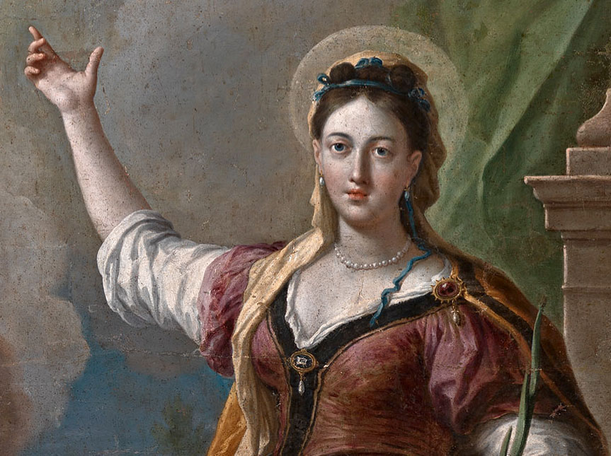
(Fig. 1.1) Before and after version, applying some of the tecniques exposed in this article.
2. Gaussian sharpening
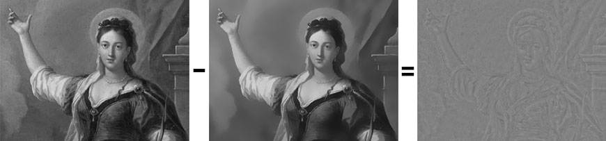
There’s plenty of resources on the web about the subject so I skip much of the basics of Photoshop USM (UnSharpMasking) and its use, why we need it, how to build masks, etc. Let me only stress again that it’s called UnSharp because it assumes the subtraction from the original picture of a blurred (unsharp) version. I’ll use a lot the “subtraction”, so here it goes a quick reminder on it, and why sharpening and blurring are close relatives inside Filter → Sharpen → Unsharp Mask…
A quick note for the reader: Grayscale images will be used throughout the article, to help us keeping the focus on tonal transitions. To mimic the effects with color pictures, use L of Lab or apply a solid white layer Color mode to have what Photoshop would consider a grayscale Luminosity version of your original. First picture (courtesy of my friend the photographer Roberto Bigano) is the starting point; then goes the blurred version and the subtraction:

(Fig. 2.1) Original picture: BW version of the painting by Paolo de Matteis “Le sante Maria, Maddalena e Dorotea” (detail) National Gallery of Cosenza, Italy (Photography © Roberto Bigano).

(Fig. 2.2) Original pictures, Blurred version and their subtraction.
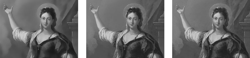
Adding the subtraction to the original makes the sharpened version:

(Fig. 2.3) Original pictures plus the difference on Fig. 2.2 gives the sharpened picture.
To do this in Photoshop, I may use offset and scaling, which makes the difference channel look more familiar:

(Fig 2.4) Using a scaled version of the difference in Photoshop.

(Fig 2.5) Detail of the sharpened version using a Gaussian Blur with Radius 4.0.
A more abstract way to visualize the effect of Gaussian Sharpening, that I personally find useful for comparison purposes, is to plot the signal intensity transition (black) and its blurred version (red), their difference (green), and the original plus the difference (thicker black):

(Fig 2.6) Intensity transition and Gaussian Sharpening.
The key concept of Gaussian Sharpening is that the difference between original and blurred version is exactly what will be enhanced. If it’s used a blurring kernel (Gaussian Blur, GB, for instance) which softens edges and texture, then edges and texture will be more prominent when the difference layer will be applied to the original. Depending on the algorithm used and the processing of the blurred picture, we may end with a sharpening that affects separately different image features.
Before going any further, let me review Photoshop’s Calculations and how to use it to sharpen. Open a picture, convert to the grayscale flavor you like the most and:
- duplicate the Gray channel twice;
- call the first ORIG and the second BLUR;
- apply a GB to BLUR
- go to the menu Image, Calculation; if you want to perform a simple subtraction: ORIG – BLUR; (Eq. 2.1)
You should setup the Calculations window as follows:

(Fig 2.7) Image – Calculations window
Pay attention that the first term of the subtraction is Source #2, and the second is Source #1 (little confusing, I know). The result you have is not scaled, and for it to be applied with the appropriate blending mode (Linear Light, LL from now on) there are two slightly different ways. Let’s baptize SS1 the Subtraction with Scale = 1 which implies a later LL blend 50% opacity, and SS2 the Subtraction with Scale = 2 which implies a later LL blend 100% opacity. Both ways are useful as we’ll see soon.

(Fig 2.8) Scaling or not the subtraction (when you perform subtraction, the result is divided by the Scale factor and added to the Offset value)
Having tested a bit more the subject, I can now affirm that SS1 (LL 50%) and SS2 (LL 100%) are not exactly the same thing, so for the sake of precision, I’m suggesting you to use SS2 only. The issues in SS1 reveals in pyramid decomposition, i.e. blacks not really black (something you can easily test); nevertheless, if you’re not in the middle of a decomposition (an image one, of course 😉 you can pick either SS1 or SS2.
3. Difference of Gaussians
Let’s shift a bit our point of view; what if, instead of subtracting a blurred version from the untouched original, the subtraction is between two differently blurred originals? Have a look to the graph before we investigate the why of such a move with GBs:

(Fig 3.1) Intensity transition and Difference of Gaussians.
The concept behind the Difference of Gaussians (DoG) is quite simple: noise is usually high frequency spatial information, and it’s blown away in both blurred version, so won’t be boosted; on the other hand the two versions keep detail in different frequency ranges. So their subtraction is a way to enhance, precisely, that frequency window:

(Fig 3.2) The subtraction between two versions of the original blurred with different radii

Fig 3.3) The original plus the difference equals the sharpened version: high frequency has not been affected by DoG (to have a gentler effect it could be suggested a lower opacity LL blend or an inverse S-shaped curve to reduce the contrast of the difference layer).

(Fig 3.4) DoG with R1=4.0 and R2=20.0 and SS2, applied LL with an extra opacity lowering at 50%.
I’m recalling here the DoG because it represent a first step off the traditional sharpening track: I can report that it’s usually applied using a blur ratio ranging from 4:1 to 5:1, while a ratio of 1.6 mimics the Laplacian of Gaussian (LoG: an operator that calculates the second derivative of signal intensity, so it’s good for instance in finding edges. I plan to add more on LoG here later on).
I still have to test it extensively: nevertheless an important feature that should be noted is its resemblance to HiRaLoAm (as Dan Margulis uses to call USM with High Radius Low Amount). But there’s a remarkable difference: namely, that edges are less or not sharpened at all, because they belong to the high frequency detail window that’s untouched by DoG (less or no difference between edges in GB1 and GB2, so less or no boosting at all).This could be a benefit in workflows where different sharpening rounds are planned and an extra step is worth its time.
4. Other blurring kernels
Since it’s clear that subtraction and blurring are the core of this kind of sharpening, I started wondering what if other kernels are used instead of, or at the same time with, GB.
Let’s take Surface Blur (SB), aka Bilateral Filter, a well known edge preserving blurring algorithm. If it keeps edges and wipes the rest out it should lead us to think: SB equal something to enhance everything but the edges. Let’s see:
(Fig 4.1) Subtraction using the edge-aware SB instead of GB.

(Fig 4.2) Affecting less the edges, the texture is more enhanced.

(Fig 4.3) The result using SB Radius = 6 and Threshold = 15.
It works as it’s supposed to do. Besides the fact that SB isn’t the fastest filter ever in the Photoshop arsenal, there are more annoying things. It’s required a bit of experience to find the correct radius/threshold couple; due to the algorithm itself, at large radii a reversion starts to appear and instead of more blurring we get more edges coming back:
(Fig 4.4) SB with Threashold 15 and radii 6.0 – 50.0 – 100.0; SB fails at larger radii and detail appears again.
A much better edge preserving filter is the Weighted Least Squares (WLS) operator. Unless you are an experienced programmer or you find the way to put your hands on a computer with MatLab and Photoshop both installed, to use it is quite a problem.The results are remarkable indeed, check the links at the bottom of the page.
5. Combined use of different blurring kernels
Here I would like to suggest the joined use of a GB and SF filters (i.e. two kernels which differs in their edge-awareness) in order to modulate the sharpening. I’m going to write some very simple and very unorthodox math; being O the Original picture, T and E respectively the Texture and Edge features of the picture (both belonging to the high frequency spatial range) we’ve seen that:
GB = O – (T+E); (Eq. 5.1)
SB = O – T; (Eq. 5.2)
A subtraction gives the Edge only component:
(SB – GB) = O – T – O + T + E = E; (Eq. 5.3)
While, rearranging the second equation, we prove that Texture is boosted by SB:
(O – SB) = T; (Eq. 5.4)
This should give us all the instruments needed to modulate the sharpening in texture and edges separately, via subtraction layers/channels to be blended in LL mode. Let’s see. Following images are GB, SB versions and the scaled subtractions we’ve talked about.

(Fig 5.1) Subtraction between SB (Radius=6 Threshold=15) and GB (Radius=4) to get an edge-only enhancement channel.

(Fig 5.2) Edge-enhancing channel applied to the original LL 50% opacity.

(Fig. 5.3) The result using SB (Radius = 6 and Threshold = 15) and GB (Radius = 4).
What we should see is a Edges only sharpening. So we’ve been able to get a Texture and Edges sharpening (with GB), a Texture only sharpening (with SB) and an Edges only sharpening (using SB -GB). More pronounced effect can be obtained by higher opacity of the LL layers (when possible) or a sigmoid (aka S-shaped) curves adjustment layer clipped to it, whose opacity can be tweaked as well. In the ToDo list there are actions/scripts (and even a Photoshop CS4 panel) to automate the process.
6. Image decomposition
Until now we’ve tried to modulate the sharpening into the same, high frequency range (edges, texture). But an image usually contains several different frequencies: higher ones correspond to finer detail (hair, for instance), lower ones to large, smoother tonal transitions (like the cheeks in a portrait). Now it’s time to try to target those different frequency ranges with appropriate, different sharpening. Pyramid decomposition is just… a way to decompose an image into several frequency ranges, and that makes easier to achieve our end.
Very simple math lies under image decomposition. I’ll use GB filter (so I’ll build a Gaussian Pyramid of 3 levels, but you can extend it to as many levels as you like); being O the Original picture, GBn(O) the GB filter applied to O with radius increasing with n:
U0 = O; (Eq. 6.1)
U1 = GB1(O); (Eq. 6.2)
U2 = GB2(O); (Eq. 6.3)
U3 = GB3(O); (Eq. 6.4)
We define differences Dn as follows:
D1 = U0 – U1; (Eq. 6.5)
D2 = U1 – U2; (Eq. 6.6)
D3 = U2 – U3; (Eq. 6.7)
So the image can be decomposed into:
O = U3 + D1 + D2 + D3; (Eq. 6.8)
In fact, substituting all the elements we get:
O = U3 + U0 – U1 + U1 – U2 + U2 – U3 = U0 = O; (Eq. 6.9)
Let’s switch to Photoshop and try to build this pyramid. We only need to perform GB filtering and subtractions, something we should be familiar with, by now.
The three GB radius will define the frequency range: I’ve chosen small radii (i.e. 1px, 5px, 15px) because the original picture is quite small; depending on the resolution of yours, they may vary. I can suggest you to select the smaller radius as the one you would use when applying conventional USM filter, the larger one corresponding to HiRaLoAm radius, and the middle one, guess what, somewhere in between. Here are the three U1, U2, U3 and the D1, D2, D3 as we defined them (I’m using SS2):

(Fig. 6.1) U1, U2 and U3, i.e. GBn(O).

(Fig 6.2) D1 = U0 – U1.

(Fig 6.3) D2 = U1 – U2.

Fig 6.4) D3 = U2 – U3.
Having all the elements, it’s now time to compose the pyramid on the Layers palette.You should make a new Set which contains bottom-up: the most blurred version U3, then D1, D2, D3, all the three LL mode, 100% opacity (remember, I used SS2). Here is how should look like your Channels and Layers palette:

(Fig 6.5) Channels and Layers palettes after filtering, subtractions and recomposing.
Don’t feel afraid by the mess here, it’s possible to automate everything (ToDo list +1) and end up with a nice tidy Channels palette. Switching on and off the Set should make no difference – and hence the decomposition works: great! So what?
7. A sharpening equalizer
Our recently decomposed picture still smells good, and moreover offers the possibility to build a 3-sliders sharpening equalizer very quickly (to add as many sliders as you want, just increase the numbers of the decomposition levels). If you made the subtractions SS1 then LL blend 50% you can already play with opacity sliders to boost high, middle and low frequencies at the same time. Personally, I find more customizable to clip a rough S-shaped curve adjustment layer to each of the Dn layers and drag those opacity sliders:

(Fig 7.1) The S-Shape curve common to all the three adjustment layers clipped to the Dn ones: their opacity control the sharpening in the High, Middle and Low Frequency range defined by the GB radius (0.5, 2.0, 4.0 for those small thumbnails).The Layers palette in its final configuration.
It reminds me the KPT Equalizer plugin (well, surely it lacks its peculiar looking UI): you can go negative, so not sharpening but smoothing a frequency range, via lowering the opacity under 50% if you used SS1 or lowering the opacity of the Dn layers in SS2. Let’s make a version:

(Fig 7.2) One of the several possibilities obtained playing with frequency sharpening sliders.
8. Bilateral and WLS Pyramids
We are allowed to use different blurring kernels, the equations of pyramid decomposition still work. Get a look, for instance, to the better SB:

(Fig 8.1) SB1(O) (Radius=2;Threshold=6), SB2(O) (R=3,T=10), SB3(O) (R=7,T=15)

(Fig 8.2) Difference layers D1, D2, D3 (I used SS1 to make them more evident).

(Fig 8.3) Result with Bilateral Pyramid decomposition for sharpening.
Can you spot the difference between Bilateral (read: which uses SB) and Gaussian pyramid equalizers? Maybe not that much here, but if you’ll use one of your (high res, maybe high bit-depth) pictures, you’ll find that being edge-aware, the Bilateral pyramid shows little or no halos, which is quite a remarkable feature in my opinion. Shadow/Highlights with SB (instead of GB) in its “engine” gives the same halo-free look by the way.
As I’ve said before,WLS filter is a much better edge-aware smoothing operator, therefore it can be used for even better enhancements (have a look to the website of WLS’ creators for examples). Adobe, anyone listening?
9. Mixed Pyramids
Strangely enough if you will, we’re allowed to mix blurring kernels and still the equations work. If you remember: 5. Combined use of different blurring kernels, I’ve found out that:
(SB – GB) = E; (Eq. 9.1)
If we modify the assumptions of the Pyramid decomposition as follows:
U0 = O; (Eq. 9.2)
U1 = SB1(O); (Eq. 9.3)
U2 = GB1(O); (Eq. 9.4)
we end up with a 2 level decomposition with:
D1 = U0 – U1 =O – SB1(O) = T; (Eq. 9.5)
Like we know from eq. 5.4.We then have:
D2 = U1 – U2 =SB1(O) – GB1(O) = E; (Eq. 9.6)
which comes from eq. 5.3. So, D1 is a frequency layer of a mixed decomposition which contains, and hence will be able to enhance,Texture alone; and D2 is a frequency layer of a mixed decomposition which contains, and hence will be able to enhance, Edges alone.
Here are the difference layers:

(Fig 9.1) O – SB1(O) = D1, the texture only detail layer (SB Radius=3,Threshold=16).

(Fig 9.2) SB1(O) – GB1(O) = D2, the edge only detail layer (GB Radius=2).
I’ll show you the full Channels and Layers palettes:

(Fig 9.3) Channels and Layers palettes of a Mixed Pyramid.
Then I’ll add the same curve adjustments layer clipped to the Dn and play with sliders. Here is an example version:

10. (temporary) Conclusions
I’ve tried to collect here material coming from various sources and my own findings around the (very personal indeed) subject of sharpening. I was particularly interested in showing how to mix blurring kernels and why pyramid decomposition is a platform on the top of which many sharpening strategies can be developed successfully. Finding new ways to use old tools in order to accomplish even slightly sophisticated tasks pays for the time spent on the project. I still have many open questions, for instance how to simulate the USM’s threshold slider via channel blending (or masks, even though I’d prefer to do the masking with calculations).
Nevertheless I’m pretty happy with the results by now: using those workflows means adding a lot of extra steps, even when I’ll find the time to put together actions/scripts to automatize the monkey work; I don’t know whether someone but me would ever try to use them in production environments (it depends on the kind of production, by the way). But, again, it’s food for thoughts: I’ve always believed in knowledge sharing and plural researches, so I’m waiting for suggestions, corrections, and smarter workflows to sharpen. I plan to keep the article updated, so check for revision number at the top of the page – I have a big fat to-do list (actions, scripts, etc). Drop me an email if you like to be warned when something new appears or just want to give feedback.
Related Topics

Davide Barranca
Lives and works near Bologna, Italy.
He’s the developer of ALCE, VitaminBW, Double USM, PS Projects and Floating Adjustments.
Davide is also a color-management aware photo-retoucher, focused in color-correction and image enhancement in fine-art photography, art reproduction photography and fine-art digital printing. Interested in academic research around digital imaging, stitching, HDRI, custom filters writing.
Specialties: Pre-press, broad experience in working side by side with photographers trying to convert from artist to technical language.
You can visit his site here >
One of the best writing about the subject I’ve seen.
It’s great you share such thing.